A few years ago, a fellow Jurel (Pacific Jack Mackerel for my English-speaking readers) asked me if it was possible to get climate information at a district level from gridded data. I did not hesitate to answer “Yes!", thinking “Surely someone has thought of this… Of course there must be a library out there that intersects gridded and polygon data”. Well, there was not, or perhaps I was not using Google properly (would not be the first time).

In any case, I had to come up with a solution, and so the first version of my package “polilla” (moth in English) came to life. Nowadays this task can easily be done with R packages like “exactextractr” or “stars”, though I have not tried them myself.
Years later, a fellow Alaskan pollock had the same request. Climate data at district level. This time I felt more confident to do it because I knew about the new packages mentioned earlier. However, I encountered a little tiny small problem. You see, for this task I have access to one of the most powerful and chunky computers for research purposes. But that’s the catch, I only have access to it, which means I cannot install R packages that require new software or system libraries. This made it “impossible” for me to test the new packages.
For the record, I could have asked the admins to install the required libraries, but I only have enough courage to talk to the fellow fish sitting 3 meters away from me. Also, I could have used Python, but despite knowing how to handle it, I despise any kind of nope ropes… I am a fish after all…
So, defeated and depressed, I decided it was time to dust off my old polilla
package and make it useful again since it did not require installing anything
extra.
It was not yet a polilla, but a cocoon
This is what my package used to do:
- Using latitude and longitude coordinates as centroids, it created a mesh or grid of square polygons.
- It overlapped the grid with another polygon (like a district) and calculated the intersected fraction of the area (useful for weighted averages).
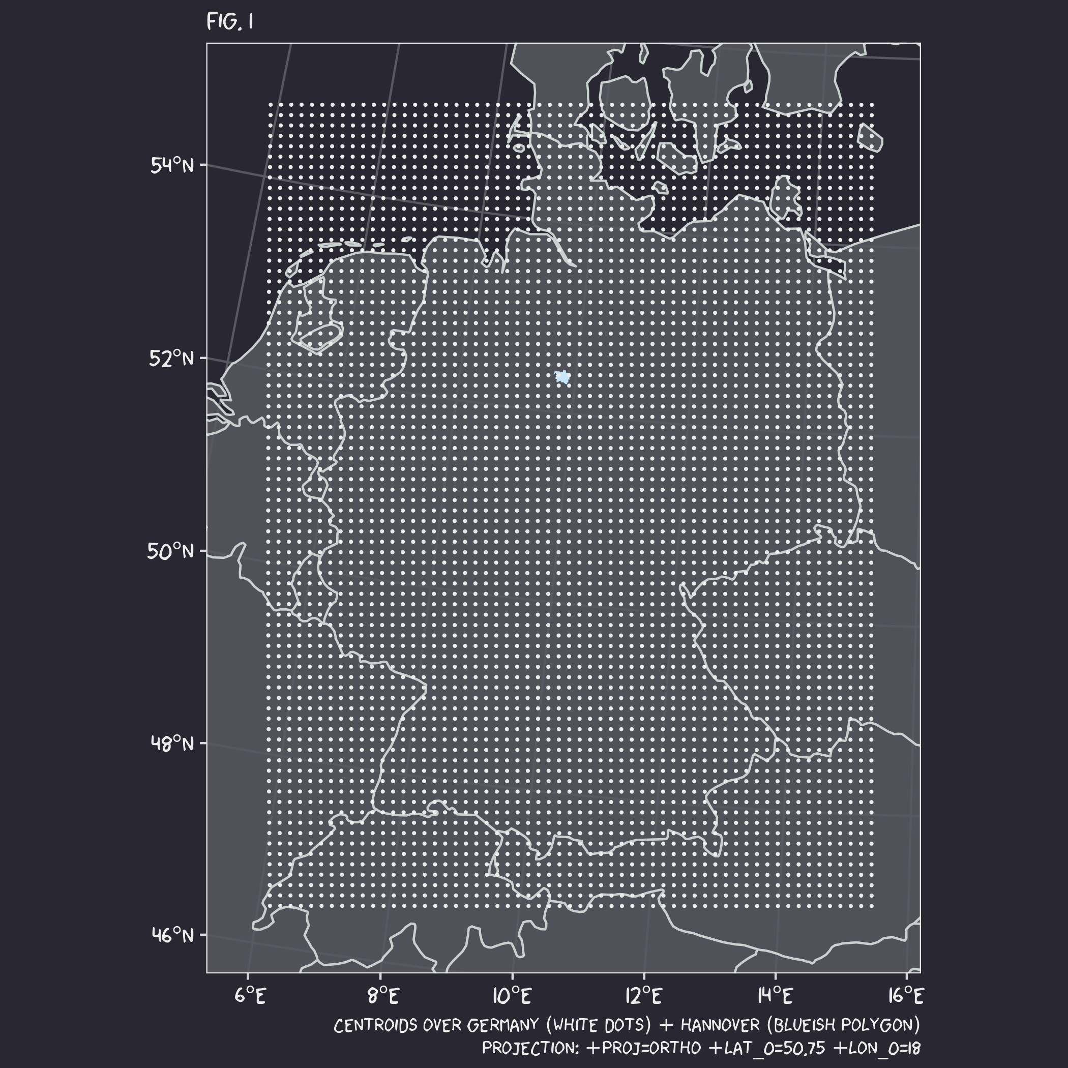
Very simple and it just worked. Unfortunately, I could not use it because my package expected the classic WGS84 longitude/latitude projection, but my data was in a weird projection called “rotated pole”. To put it simply, this projection sets the pair of coordinates (0°, 0°) somewhere in Europe to make the grid centers in Europe “equally” spaced. There is no need to dig too deeply into this, but if you are curious, this is an example of what the centroids look like in the rotated pole projection.
Starting the metamorphosis
Fixing the projection issue was quite simple, all I had to do was add an extra argument to each function so that I could pass any projection I wanted. Then you might think that updating the functions should be enough, right? I just need to pass the right projection, right?
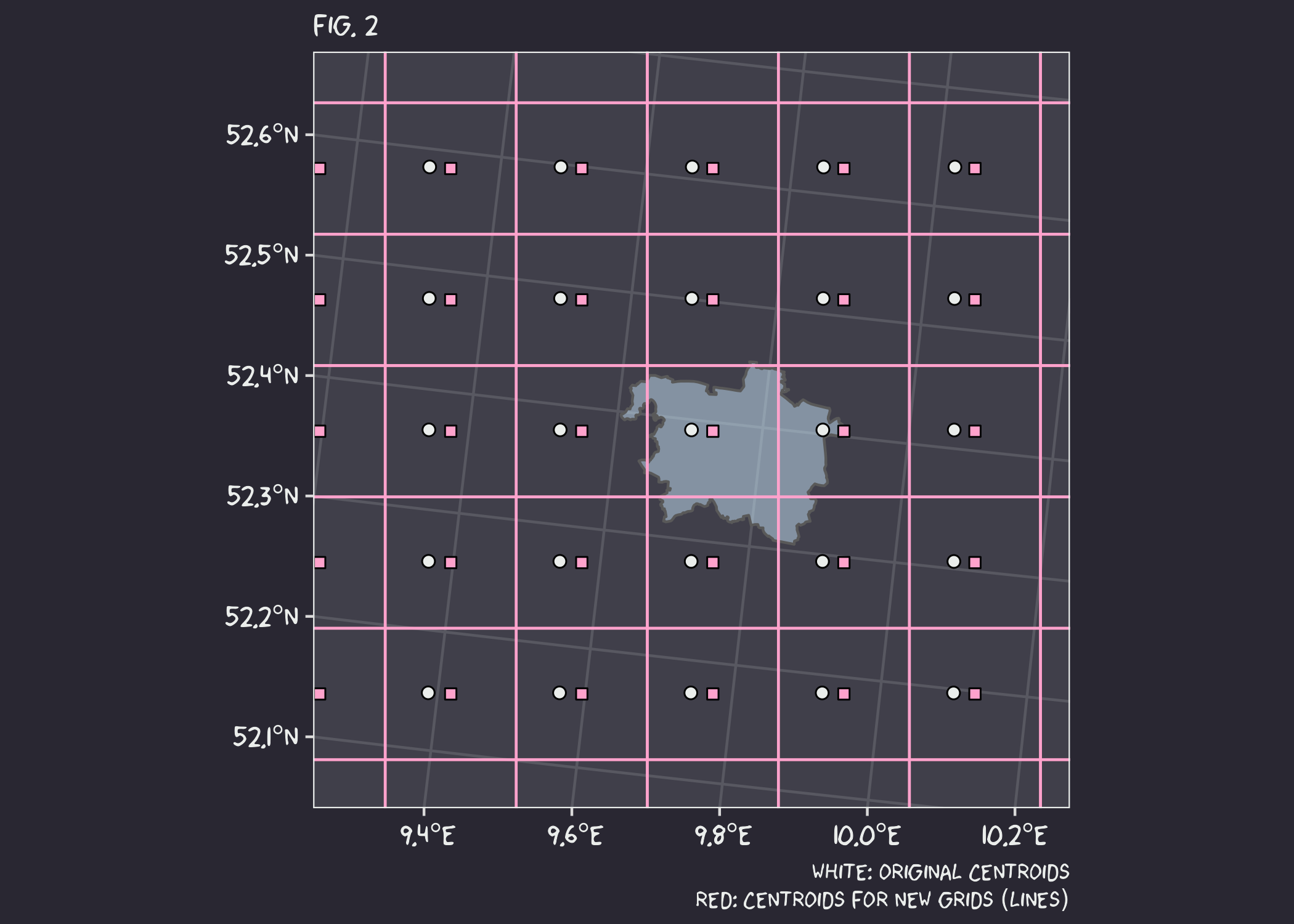
Uhmm… that did not work as planned. The centroids of the new grid (red squares) should be at the same position as the original coordinates (white circles). Instead, there is a strange offset.
After hours and hours of swimming in circles, I realised what the problem was. If you have been paying attention, you might remember something about the grids being “equally” spaced. Well, the original coordinates are indeed equally spaced, but in degrees. The moment I transformed the centroids to this rotated pole projection, the coordinates were converted to meters, thus making them not equally spaced. This is not an error or a bug, it is just the way projections work and why they are a pain in the tail.
I do not know if this can be fixed by working in degrees instead of meters, but at least I had found a way to reduce the offset (and improve performance!). You see, the further away the centroids are from the origin (0°, 0°), the greater the distance between them and the greater the offset. But by creating the grid on a smaller area (say the boundaries of the city of Hanover), the distance between the centroids remains relatively constant compared to using the whole country.
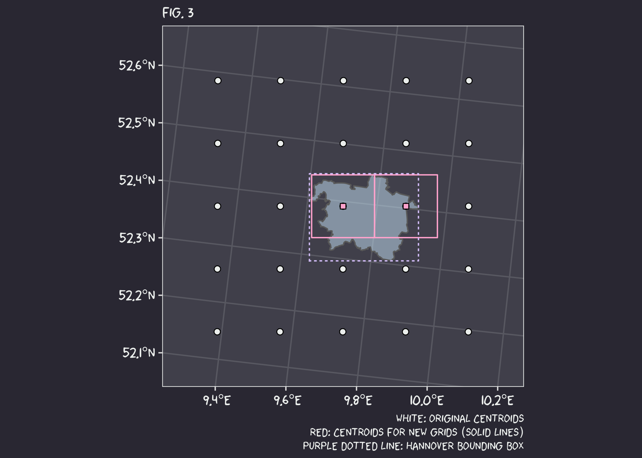
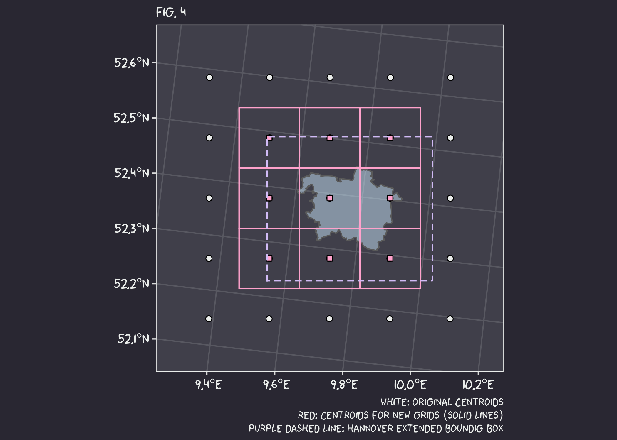
OK, it worked, but we have another problem. Simply using the bounding box of the desired polygon (Fig 3. - purple dotted line) to select the desired grids is not enough. This is because the bounding box only intersects the grid centroids, not the area covered by the grid itself. I could create the grid first and then do the selection, but I would be back to the problem of mismatched centroids. Instead, I can just extend the bounding box by half the resolution of the grid cells (Fig. 4 - new purple dashed line).
Nice… Now the final step is to calculate the intersection area between the
grids and the reference polygon. Based on this, we can also calculate the
weights in case we want to use them for spatial statistics (like averages for
the whole district). This can easily be done with functions from the sf
package.
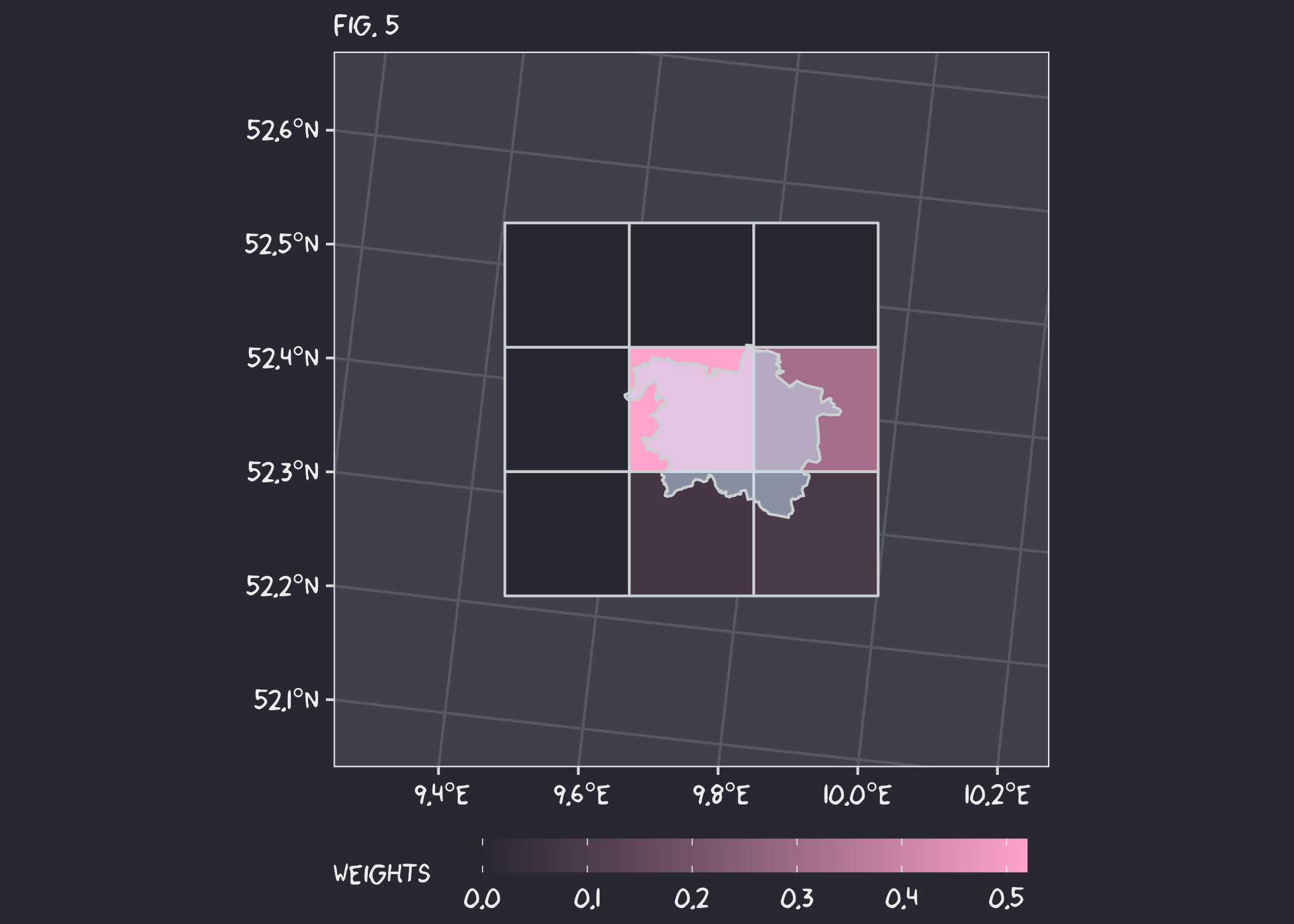
It is a beautiful… moth…
And it is done. Having the weights for each grid cell is enough to get area averaged climate values for different districts. As I said before, this can be done with other packages but, this is just another option.
On a more personal note, this makes me understand much better why projections
are so important and that things do not have to be perfect to be
useful. I cannot say that the grids produced by polilla are accurate, as
it assume an equally spaced grid when in fact it is not. However, the error
is so small that it makes no difference to the spatial statistics.
Now fly, you ugly moth.